8. 木構造とアンサンブル学習

本章では、第 7 章で扱ったロジスティック回帰や k-近傍法、SVM に続く分類手法として、決定木 とそれを発展させた アンサンブル学習(ランダムフォレスト・勾配ブースティング)を学びます。
8.1 決定木
8.1.1 決定木とは
決定木(Decision Tree) は、データを「木構造」で分類・回帰するアルゴリズムです。if-then ルールの集まりとして表現され、人間が理解しやすいのが特徴です。
graph TB
    A("花弁の長さ ≤ 2.5cm?") -->|Yes| B("Setosa")
    A -->|No| C("花弁の幅 ≤ 1.7cm?")
    C -->|Yes| D("Versicolor")
    C -->|No| E("Virginica")

    classDef data fill:#D9EAF3,stroke:#0072B2,stroke-width:2px,color:#000
    classDef proc fill:#D9F0EA,stroke:#009E73,stroke-width:2px,color:#000
    class A,C data
    class B,D,E proc
決定木の特徴
- 解釈性が高い:ルールが明確で説明しやすい
- 非線形:複雑な境界を表現できる
- 前処理不要:標準化やダミー変数化が不要
- 過学習しやすい:深くしすぎると訓練データに過度に適合
8.1.2 決定木の仕組み
決定木は、データを「分割」していくことで分類を行います。情報利得(Information Gain) や ジニ不純度(Gini Impurity) という指標を使って、最も効果的な分割方法を選びます。
ジニ不純度
ジニ不純度は、データの「混ざり具合」を表す指標です。
- 完全に1つのクラスだけ → ジニ不純度 = 0(純粋)
- クラスが均等に混ざっている → ジニ不純度が大きい(不純)
決定木は、ジニ不純度が小さくなるように分割を繰り返します。
8.1.3 決定木の実装
決定木を実装するには、sklearn.tree.DecisionTreeClassifier クラスを使用します。学習した木の構造は sklearn.tree.plot_tree() 関数で可視化できます。
import numpy as np
from sklearn.tree import DecisionTreeClassifier, plot_tree
from sklearn.model_selection import train_test_split
from sklearn.metrics import accuracy_score, classification_report
import seaborn as sns
import matplotlib.pyplot as plt

# アヤメデータセットの読み込み
iris = sns.load_dataset('iris')

# 特徴量とラベルの分離
X = iris[['petal_length', 'petal_width']].values
y = iris['species'].values

# データ分割
X_train, X_test, y_train, y_test = train_test_split(
    X, y, test_size=0.2, random_state=42
)

# 決定木モデルの学習(最大深さ3)
model = DecisionTreeClassifier(max_depth=3, random_state=42)
model.fit(X_train, y_train)

# 予測と評価
y_pred = model.predict(X_test)
accuracy = accuracy_score(y_test, y_pred)
print(f"精度: {accuracy:.2%}")

# 決定木の可視化
plt.figure(figsize=(12, 8))
plot_tree(model, feature_names=['petal_length', 'petal_width'],
          class_names=['setosa', 'versicolor', 'virginica'], filled=True)
plt.show()
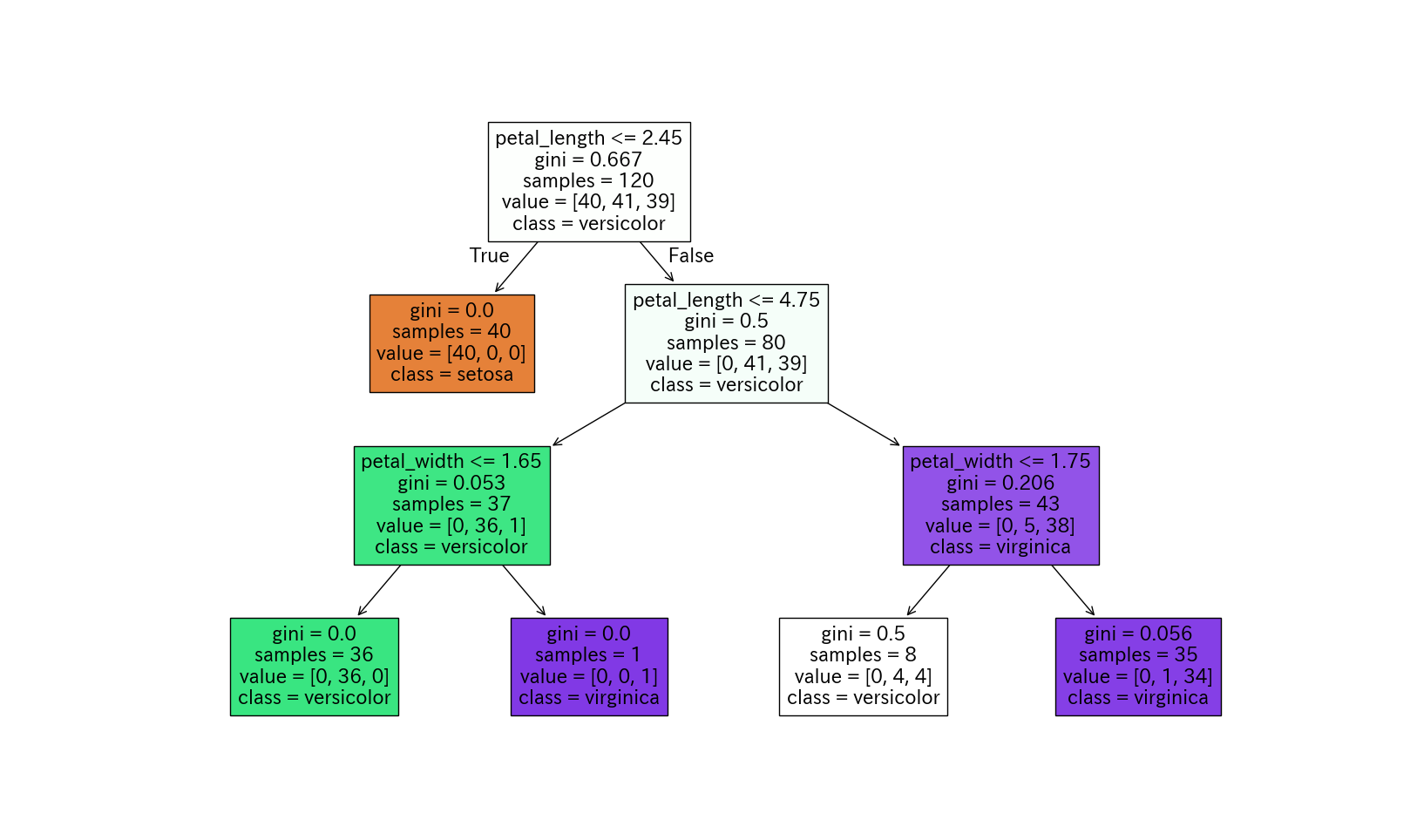
8.1.4 決定木のハイパーパラメータ
決定木の性能を調整するための主なハイパーパラメータは、以下になります。
| パラメータ | 説明 | 影響 |
|---|---|---|
max_depth |
木の最大深さ | 小さい→シンプル、大きい→複雑 |
min_samples_split |
分割に必要な最小サンプル数 | 大きい→シンプル |
min_samples_leaf |
葉ノードの最小サンプル数 | 大きい→シンプル |
決定木の過学習
max_depth=None(深さ制限なし)にすると、訓練データに完全に適合してしまい、テストデータでの性能が悪化します(過学習)。適切な深さは、交差検証などで決定します。
Playground:決定木
決定木 の Playground では、max_depth のスライダーを動かすと決定領域と木の構造が同時に変わります。区切りが必ず軸に平行になるため境界が階段状になること、深さ 1〜2 では大まかに、深さ 5〜6 では点ひとつのために細かく区切られていく(=過学習)様子を確かめてみましょう。
8.2 ランダムフォレスト
8.2.1 ランダムフォレストとは
ランダムフォレスト(Random Forest) は、複数の決定木を組み合わせたアンサンブル学習(集団学習) の一種です。
graph TB
    A("訓練データ") --> B1("決定木 1")
    A --> B2("決定木 2")
    A --> B3("決定木 3")
    A --> B4("...")
    A --> B5("決定木 N")

    B1 --> C("投票 / 平均")
    B2 --> C
    B3 --> C
    B4 --> C
    B5 --> C

    C --> D("最終予測")

    classDef data fill:#D9EAF3,stroke:#0072B2,stroke-width:2px,color:#000
    classDef proc fill:#D9F0EA,stroke:#009E73,stroke-width:2px,color:#000
    classDef out fill:#F5ECE2,stroke:#BF8040,stroke-width:2px,color:#000
    class A data
    class B1,B2,B3,B4,B5 proc
    class C,D out
ランダムフォレストの特徴
- 高精度:単一の決定木より高い精度
- 過学習に強い:複数の木の平均を取るため
- 特徴量の重要度:どの特徴量が重要かが分かる
- 並列化が可能:各木を独立に学習できる
8.2.2 ランダムフォレストの仕組み
ランダムフォレストは以下の手順で動作します。
- ブートストラップサンプリング:訓練データからランダムにサンプリング(重複あり)
- ランダムな特徴量選択:各分割でランダムに特徴量のサブセットを選択
- 複数の決定木を学習:それぞれ異なるデータ・特徴量で学習
- 予測を集約:分類は多数決として捉えられますが、scikit-learn の
RandomForestClassifierクラスは各木が出すクラス確率を平均し、最大のクラスを選びます。回帰では各木の予測値を平均します。
ランダム性を入れることによる恩恵
- 多様性:各決定木がさまざまなパターンを学習
- 汎化性能:特定のデータへの過度な適合を防ぐ
- ロバスト性:一部の木が間違えても、他の木が補える
8.2.3 ランダムフォレストの実装
ランダムフォレストを実装するには、sklearn.ensemble.RandomForestClassifier クラスを使用します。
from sklearn.ensemble import RandomForestClassifier
from sklearn.model_selection import train_test_split
from sklearn.metrics import accuracy_score, classification_report
import seaborn as sns

# アヤメデータセットの読み込み
iris = sns.load_dataset('iris')

# 特徴量とラベルの分離
X = iris[['petal_length', 'petal_width']].values
y = iris['species'].values

# データ分割
X_train, X_test, y_train, y_test = train_test_split(
    X, y, test_size=0.2, random_state=42
)

# ランダムフォレストモデルの学習
model = RandomForestClassifier(n_estimators=100, max_depth=3, random_state=42)
model.fit(X_train, y_train)

# 予測と評価
y_pred = model.predict(X_test)
accuracy = accuracy_score(y_test, y_pred)
print(f"精度: {accuracy:.2%}")
print("\n分類レポート:")
print(classification_report(y_test, y_pred))
8.2.4 ランダムフォレストのハイパーパラメータ
| パラメータ | 説明 | 推奨値 |
|---|---|---|
n_estimators |
木の数 | 100〜500 |
max_depth |
各木の最大深さ | 適宜調整 |
max_features |
分割時の特徴量数 | 'sqrt'(デフォルト) |
Playground:ランダムフォレスト
ランダムフォレスト の Playground では、木の本数を 1 にすると境界はただの決定木と同じギザギザですが、本数を増やすほど多数決でならされてなめらかで安定した境界になります。色が薄い部分は木どうしの意見が割れている場所です。n_estimators を増やす意味を目で確かめてみましょう。
8.3 勾配ブースティング
発展トピック
本節は アンサンブルにはバギング系(並列)とブースティング系(直列)の二系統がある という大枠の理解を目的とした発展トピックです。実装の詳細より「ランダムフォレストとの違い」を押さえておきましょう。
8.3.1 勾配ブースティングとは
勾配ブースティング(Gradient Boosting) は、複数のモデルを順番に学習させるアンサンブル手法です。それまでのモデル(木)を合わせた予測の誤差(残差)を、次のモデルが修正していくように学習します。
graph LR
    A("データ") --> B("モデル 1")
    B --> C("残差 1")
    C --> D("モデル 2")
    D --> E("残差 2")
    E --> F("モデル 3")
    F --> G("...")
    G --> H("最終予測")

    classDef data fill:#D9EAF3,stroke:#0072B2,stroke-width:2px,color:#000
    classDef proc fill:#D9F0EA,stroke:#009E73,stroke-width:2px,color:#000
    classDef out fill:#F5ECE2,stroke:#BF8040,stroke-width:2px,color:#000
    classDef neu fill:#F2F2F2,stroke:#8C8C8C,stroke-width:2px,color:#000
    class A,C,E data
    class B,D,F proc
    class H out
    class G neu
勾配ブースティングの特徴
- 高精度:多くのコンペで優勝実績あり
- 過学習しやすい:適切な正則化が必要
- 学習が遅い:順番に学習するため並列化が難しい
8.3.2 勾配ブースティングの実装
scikit-learn では sklearn.ensemble.GradientBoostingClassifier クラスを使用します。
from sklearn.ensemble import GradientBoostingClassifier
from sklearn.model_selection import train_test_split
from sklearn.metrics import accuracy_score
import seaborn as sns

# データ準備
iris = sns.load_dataset('iris')
X = iris.drop('species', axis=1).values
y = iris['species'].values

X_train, X_test, y_train, y_test = train_test_split(
    X, y, test_size=0.2, random_state=42
)

# 勾配ブースティングモデルの学習
model = GradientBoostingClassifier(n_estimators=100, learning_rate=0.1, random_state=42)
model.fit(X_train, y_train)

# 予測と評価
y_pred = model.predict(X_test)
accuracy = accuracy_score(y_test, y_pred)
print(f"精度: {accuracy:.2%}")
8.3.3 XGBoost と LightGBM
実務では、勾配ブースティングを高速かつ高機能に実装した XGBoost や LightGBM がよく使われます。それぞれ xgboost.XGBClassifier クラスと lightgbm.LGBMClassifier クラスを使用します。これらは scikit-learn とは独立した別パッケージなので、使用前にインストールが必要です。
# XGBoost の例
from xgboost import XGBClassifier

model = XGBClassifier(n_estimators=100, learning_rate=0.1, random_state=42)
model.fit(X_train, y_train)
# LightGBM の例
from lightgbm import LGBMClassifier

model = LGBMClassifier(n_estimators=100, learning_rate=0.1, random_state=42)
model.fit(X_train, y_train)
どれを使うべきか
- RandomForest:シンプルで扱いやすい、並列化可能
- GradientBoosting:基本的な勾配ブースティング
- XGBoost:高速・高精度、Kaggle で人気
- LightGBM:さらに高速、大規模データ向け
公式チュートリアル
本節の内容を実際に手を動かして深掘りしたい場合は、以下の公式ドキュメントを参照してください。
- scikit-learn の勾配ブースティング:User Guide / Gradient Tree Boosting
- XGBoost:Tutorials(Introduction to Boosted Trees が概念入門)
- LightGBM:Quick Start / Python Quick Start Guide
Playground:勾配ブースティング
勾配ブースティング の Playground では、段数(木の本数)を増やすたびに予測の階段状の曲線がデータへ近づき、赤い残差の線が短くなっていきます。学習率を 0.05 にすると少しずつ、1.0 にすると数本で一気に fit します。「それまでの木を合わせた予測の残差を次の木が学習する」仕組みを 1 段ずつ追ってみましょう。
8.4 特徴量の重要度
8.4.1 特徴量の重要度とは
ランダムフォレストや勾配ブースティングでは、各特徴量がどれだけ予測に貢献しているかを定量的に評価できます。不純度の減少に基づく重要度は、取り得る値の種類が多い特徴量を高く評価しやすい傾向があります。必要に応じて、学習に使っていないデータで Permutation Importance も確認します。
8.4.2 特徴量の重要度の可視化
import pandas as pd
import matplotlib.pyplot as plt
from sklearn.ensemble import RandomForestClassifier
import seaborn as sns

# データ準備
iris = sns.load_dataset('iris')
X = iris.drop('species', axis=1)
y = iris['species']

# ランダムフォレストの学習
model = RandomForestClassifier(n_estimators=100, random_state=42)
model.fit(X, y)

# 特徴量の重要度
importances = model.feature_importances_
feature_names = X.columns

# DataFrameに整理
importance_df = pd.DataFrame({
    '特徴量': feature_names,
    '重要度': importances
}).sort_values('重要度', ascending=False)

print("特徴量の重要度:")
print(importance_df)

# 可視化
plt.figure(figsize=(8, 5))
plt.barh(importance_df['特徴量'], importance_df['重要度'])
plt.xlabel('重要度')
plt.title('特徴量の重要度')
plt.gca().invert_yaxis()
plt.show()
特徴量の重要度の活用
- 特徴量選択:重要度の低い特徴量を削除してモデルを簡略化
- データ収集の優先順位:重要な特徴量を優先的に収集
- ビジネス理解:どの要因が重要かを理解
8.5 発展: 異種モデルのアンサンブル
8.5.1 異種モデルを組み合わせる発想
ランダムフォレストや勾配ブースティングは「同じ種類のモデル(決定木)」を複数組み合わせるアンサンブルでした。これに対し、異なる系統のモデル(例:ロジスティック回帰・SVM・ランダムフォレスト)を組み合わせることもできます。各モデルが異なる「クセ」を持つため、組み合わせることで個々より安定した予測が得られる場合があります。
graph LR
    A("訓練データ") --> B("ロジスティック回帰")
    A --> C("SVM")
    A --> D("ランダムフォレスト")
    B --> E("投票 / 確率平均")
    C --> E
    D --> E
    E --> F("最終予測")

    classDef data fill:#D9EAF3,stroke:#0072B2,stroke-width:2px,color:#000
    classDef proc fill:#D9F0EA,stroke:#009E73,stroke-width:2px,color:#000
    classDef model fill:#F7EBF2,stroke:#CC79A7,stroke-width:2px,color:#000
    classDef out fill:#F5ECE2,stroke:#BF8040,stroke-width:2px,color:#000
    class A data
    class E proc
    class B,C,D model
    class F out
scikit-learn では以下の 2 つが代表的です。
VotingClassifier:各モデルの予測を多数決(hard)または確率平均(soft)で集約StackingClassifier:各モデルの予測を入力として、別の「メタ学習器」がもう一度学習
8.5.2 VotingClassifier
sklearn.ensemble.VotingClassifier クラスを使います。estimators に「(名前, モデル)」のタプルのリストを渡し、voting='hard'(多数決)または voting='soft'(確率平均)を指定します。標準化が必要なモデル(LR・SVM)は sklearn.pipeline.make_pipeline() 関数で StandardScaler クラスと一緒に包んでおくと、fit() メソッドの実行時に自動で標準化されます。
from sklearn.linear_model import LogisticRegression
from sklearn.ensemble import RandomForestClassifier, VotingClassifier
from sklearn.svm import SVC
from sklearn.preprocessing import StandardScaler
from sklearn.pipeline import make_pipeline
from sklearn.model_selection import train_test_split
from sklearn.metrics import accuracy_score
import seaborn as sns

iris = sns.load_dataset('iris')
X = iris[['sepal_length', 'sepal_width']].values
y = iris['species'].values

X_train, X_test, y_train, y_test = train_test_split(
    X, y, test_size=0.2, random_state=42
)

# 標準化が必要なモデルは Pipeline で包む
lr = make_pipeline(StandardScaler(),
                   LogisticRegression(max_iter=1000, random_state=42))
svm = make_pipeline(StandardScaler(),
                    SVC(kernel='rbf', C=1.0, gamma='scale',
                        probability=True, random_state=42))
rf = RandomForestClassifier(n_estimators=100, max_depth=3, random_state=42)

# 異種モデルを多数決(soft voting)で結合
voting = VotingClassifier(
    estimators=[('lr', lr), ('svm', svm), ('rf', rf)],
    voting='soft'
)
voting.fit(X_train, y_train)
print(f"Voting (soft) 精度: {accuracy_score(y_test, voting.predict(X_test)):.2%}")
hard vs soft voting
- hard voting:各モデルが「最終的な予測クラス」を出して多数決
- soft voting:各モデルが「クラス確率」を出し、その平均値が最大のクラスを採用
soft voting の方が情報量が多く、一般に精度が高い傾向。ただし SVM では SVC(probability=True) の指定が必要です(確率を出すために内部で交差検証を行うため、学習がやや重くなります)。
8.5.3 StackingClassifier
sklearn.ensemble.StackingClassifier クラスはさらに発展した手法で、複数モデルの予測を「特徴量」として、上に積み上げた メタ学習器(通常はロジスティック回帰)が最終的な予測を行います。Kaggle などのコンペで上位入賞者がよく使う手法です。
graph LR
    A("訓練データ") --> B("ベース<br/>モデル群")
    B --> C("各モデルの予測<br/>= 新しい特徴量")
    C --> D("メタ学習器<br/>例: LR")
    D --> E("最終予測")

    classDef data fill:#D9EAF3,stroke:#0072B2,stroke-width:2px,color:#000
    classDef model fill:#F7EBF2,stroke:#CC79A7,stroke-width:2px,color:#000
    classDef out fill:#F5ECE2,stroke:#BF8040,stroke-width:2px,color:#000
    class A,C data
    class B,D model
    class E out
Voting と Stacking の使い分け
- Voting:シンプルで導入しやすい、計算も軽い
- Stacking:メタ学習器に「どのモデルをどれだけ信用するか」を学ばせる (性能上限は高いが、過学習リスクと計算コストも増える)
どちらも VotingClassifier(estimators=..., voting='soft') / StackingClassifier(estimators=..., final_estimator=LogisticRegression()) という形で、異種モデルを 1 つの fit() メソッド / predict() メソッドで扱える のが scikit-learn の便利な点です。
8.6 モデルの比較
8.6.1 各手法の特徴まとめ
第 7 章と本章で扱った 6 つの分類手法を一覧で比較します。
| 手法 | 精度(一般的な傾向) | 解釈性 | 学習速度 | 過学習 | 標準化 |
|---|---|---|---|---|---|
| ロジスティック回帰(7 章) | 中 | 高 | 速い | しにくい | 推奨 |
| k-近傍法(7 章) | 中 | 中 | 学習は速い/予測は遅い | k に依存 | 通常必要 |
| SVM(7 章) | 高 | 低 | データ量により遅くなる | しにくい | 通常必要 |
| 決定木 | 中 | 高 | 速い | しやすい | 不要 |
| ランダムフォレスト | 高 | 中 | 普通 | しにくい | 不要 |
| 勾配ブースティング | 高 | 低 | 遅い | しやすい | 不要 |
標準化の要不要は系統で決まる
- 距離・内積を使う系(k-NN, SVM, ロジスティック回帰)→ 標準化を行う
- 木の分割を使う系(決定木, ランダムフォレスト, 勾配ブースティング)→ 標準化は不要
モデルの仕組みを思い出せば、標準化が必要かどうかは判断できます。
8.6.2 使い分けの指針
graph TB
    A("モデル選択") --> B{解釈性が重要?}
    B -->|Yes| C("決定木")
    B -->|No| D{データサイズ?}
    D -->|小〜中| E{特徴量の重要度<br/>が欲しい?}
    D -->|大| F("LightGBM / XGBoost")
    E -->|Yes| G("ランダムフォレスト")
    E -->|No| H("SVM / ランダムフォレスト")

    classDef data fill:#D9EAF3,stroke:#0072B2,stroke-width:2px,color:#000
    classDef model fill:#F7EBF2,stroke:#CC79A7,stroke-width:2px,color:#000
    class A,B,D,E data
    class C,F,G,H model
より細かい使い分けの指針
scikit-learn 公式の Choosing the right estimator は、データ量を起点に「Linear SVC → KNeighbors → SVC → アンサンブル」のように試す順序を示しており、回帰・クラスタリング・次元削減もカバーしています(XGBoost / LightGBM は対象外)。本章の指針と合わせて参考にしてください。
8.7 演習問題
演習 8-1: ジニ不純度の手計算
演習 8-1
ジニ不純度について、次の場合の値を手計算で求めてください。
- クラス A が 80%、クラス B が 20% のノード
- クラス A が 50%、クラス B が 50% のノード
- クラス A が 100% のノード(純粋なノード)
解答例
ジニ不純度の定義 \(G = 1 - \sum_{k} p_k^2\) に各クラスの割合を代入します。
-
クラスA 80%、クラスB 20%
\[G = 1 - (0.8^2 + 0.2^2) = 1 - (0.64 + 0.04) = 0.32\] -
クラスA 50%、クラスB 50%
\[G = 1 - (0.5^2 + 0.5^2) = 1 - 0.5 = 0.5\] -
クラスA 100%(純粋なノード)
\[G = 1 - 1^2 = 0\]
考察:2クラスのジニ不純度は、半々のとき最大の0.5になり、片方に偏るほど小さくなります。1クラスだけになると0です。決定木は、分割後のジニ不純度が小さくなる(ノードが純粋になる)分割を選びます。
演習 8-2: 決定木による分類と過学習
演習 8-2
penguins データセットを使って、bill_length_mm・bill_depth_mm・body_mass_g の 3 つの数値特徴量からペンギンの種類(species:Adelie / Chinstrap / Gentoo)を分類する決定木を実装してください。
タスク:
- penguins データセットを読み込み、
dropna()メソッドで欠損値のある行を削除する - 特徴量
X = penguins[['bill_length_mm', 'bill_depth_mm', 'body_mass_g']]、ラベルy = penguins['species']を準備する - データを「訓練 80%、テスト 20%」(
random_state=42)に分割する - 決定木モデル
DecisionTreeClassifier(max_depth=3, random_state=42)を学習する - テストデータで予測し、正解率(accuracy)と
classification_report()関数を表示する plot_tree()関数で学習した木構造を可視化するmax_depthを 1 から 10 まで変化させ、訓練精度とテスト精度をグラフにプロットする- 過学習が始まる
max_depthはいくつか考察する
import seaborn as sns
import matplotlib.pyplot as plt
from sklearn.tree import DecisionTreeClassifier, plot_tree
from sklearn.model_selection import train_test_split
from sklearn.metrics import accuracy_score, classification_report

# 1. データの読み込みと欠損値の削除

# 2. 特徴量 X とラベル y の設定

# 3. 訓練・テストに分割(8:2, random_state=42)

# 4. 決定木モデル(max_depth=3)の学習

# 5. テストデータで予測し、正解率と classification_report を表示

# 6. plot_tree で木構造を可視化

# 7. max_depth を 1〜10 で変化させ、訓練精度とテスト精度をプロット
解答例
import seaborn as sns
import matplotlib.pyplot as plt
from sklearn.tree import DecisionTreeClassifier, plot_tree
from sklearn.model_selection import train_test_split
from sklearn.metrics import accuracy_score, classification_report

# 1. データの読み込みと欠損値の削除
penguins = sns.load_dataset("penguins").dropna()

# 2. 特徴量 X とラベル y の設定
X = penguins[["bill_length_mm", "bill_depth_mm", "body_mass_g"]]
y = penguins["species"]

# 3. 訓練・テストに分割(8:2, random_state=42)
X_train, X_test, y_train, y_test = train_test_split(
    X, y, test_size=0.2, random_state=42
)

# 4. 決定木モデル(max_depth=3)の学習
model = DecisionTreeClassifier(max_depth=3, random_state=42)
model.fit(X_train, y_train)

# 5. テストデータで予測し、正解率と classification_report を表示
y_pred = model.predict(X_test)
print(f"正解率: {accuracy_score(y_test, y_pred):.4f}")
print(classification_report(y_test, y_pred))

# 6. plot_tree で木構造を可視化
plt.figure(figsize=(14, 8))
plot_tree(model, feature_names=X.columns, class_names=model.classes_,
          filled=True, fontsize=9)
plt.show()

# 7. max_depth を 1〜10 で変化させ、訓練精度とテスト精度をプロット
depths = range(1, 11)
train_accs, test_accs = [], []
for depth in depths:
    clf = DecisionTreeClassifier(max_depth=depth, random_state=42)
    clf.fit(X_train, y_train)
    train_accs.append(accuracy_score(y_train, clf.predict(X_train)))
    test_accs.append(accuracy_score(y_test, clf.predict(X_test)))
    print(f"max_depth={depth:2d}: 訓練 {train_accs[-1]:.4f}, "
          f"テスト {test_accs[-1]:.4f}")

plt.figure(figsize=(8, 5))
plt.plot(depths, train_accs, marker="o", label="訓練精度")
plt.plot(depths, test_accs, marker="s", label="テスト精度")
plt.xlabel("max_depth")
plt.ylabel("正解率")
plt.legend()
plt.grid(True, alpha=0.3)
plt.show()
正解率: 0.9851
              precision    recall  f1-score   support

      Adelie       0.97      1.00      0.98        31
   Chinstrap       1.00      0.92      0.96        13
      Gentoo       1.00      1.00      1.00        23

    accuracy                           0.99        67
   macro avg       0.99      0.97      0.98        67
weighted avg       0.99      0.99      0.98        67

max_depth= 1: 訓練 0.7669, テスト 0.7015
max_depth= 2: 訓練 0.9511, テスト 0.9254
max_depth= 3: 訓練 0.9699, テスト 0.9851
max_depth= 4: 訓練 0.9850, テスト 1.0000
max_depth= 5: 訓練 0.9925, テスト 0.9701
max_depth= 6: 訓練 0.9962, テスト 0.9701
max_depth= 7: 訓練 1.0000, テスト 0.9701
max_depth= 8: 訓練 1.0000, テスト 0.9701
max_depth= 9: 訓練 1.0000, テスト 0.9701
max_depth=10: 訓練 1.0000, テスト 0.9701
実行すると、まず深さ3の木構造が表示されます。根ノードでは bill_depth_mm による分割が選ばれ、くちばしが薄く体重の重いグループとして Gentoo が早い段階で分離されます。続いて、max_depth に対する訓練精度・テスト精度の折れ線グラフが表示されます。
考察:深さ1では訓練・テストとも7割程度で、未学習です。深さ2〜3で精度が大きく上がり、テスト精度は深さ4で1.0000になります。深さ5以降は訓練精度が1.0に近づく一方、テスト精度は0.9701に下がっており、過学習です。このデータでは深さ3〜4が適切です。
演習 8-3: ランダムフォレストと特徴量の重要度
演習 8-3
演習 8-2 と同じ penguins データセットの設定で、ペンギンの種類を分類するランダムフォレストを実装してください。また、特徴量の重要度を確認し、決定木との違いを考察してください。
タスク:
- 演習 8-2 と同様に、データの読み込みから訓練・テスト分割までを行う
- ランダムフォレスト
RandomForestClassifier(n_estimators=100, max_depth=3, random_state=42)を学習し、テストデータの正解率を表示する feature_importances_属性を取り出し、特徴量名と一緒にpandas.DataFrameクラスにまとめて重要度の降順で表示する- 棒グラフで重要度を可視化する
max_depthを1, 2, 3, 5, Noneと変化させたときのテスト精度を比較する- 決定木(演習 8-2)と比べて何が変わったか考察する
import seaborn as sns
import pandas as pd
import matplotlib.pyplot as plt
from sklearn.ensemble import RandomForestClassifier
from sklearn.model_selection import train_test_split
from sklearn.metrics import accuracy_score

# 1. データの準備(演習 8-2 と同じ)

# 2. ランダムフォレストの学習と正解率の表示

# 3. 特徴量の重要度を DataFrame に整理して表示

# 4. 棒グラフで可視化

# 5. max_depth を変えたときのテスト精度を比較
解答例
import seaborn as sns
import pandas as pd
import matplotlib.pyplot as plt
from sklearn.ensemble import RandomForestClassifier
from sklearn.model_selection import train_test_split
from sklearn.metrics import accuracy_score

# 1. データの準備(演習8-2と同じ)
penguins = sns.load_dataset("penguins").dropna()
X = penguins[["bill_length_mm", "bill_depth_mm", "body_mass_g"]]
y = penguins["species"]
X_train, X_test, y_train, y_test = train_test_split(
    X, y, test_size=0.2, random_state=42
)

# 2. ランダムフォレストの学習と正解率の表示
model = RandomForestClassifier(n_estimators=100, max_depth=3,
                               random_state=42)
model.fit(X_train, y_train)
print(f"正解率: {accuracy_score(y_test, model.predict(X_test)):.4f}")

# 3. 特徴量の重要度を DataFrame に整理して表示
importance_df = pd.DataFrame({
    "特徴量": X.columns,
    "重要度": model.feature_importances_
}).sort_values("重要度", ascending=False)
print(importance_df)

# 4. 棒グラフで可視化
plt.figure(figsize=(8, 4))
plt.barh(importance_df["特徴量"], importance_df["重要度"])
plt.xlabel("重要度")
plt.gca().invert_yaxis()
plt.show()

# 5. max_depth を変えたときのテスト精度を比較
for depth in [1, 2, 3, 5, None]:
    clf = RandomForestClassifier(n_estimators=100, max_depth=depth,
                                 random_state=42)
    clf.fit(X_train, y_train)
    acc = accuracy_score(y_test, clf.predict(X_test))
    print(f"max_depth={str(depth):>4s}: テスト精度 {acc:.4f}")
正解率: 1.0000
              特徴量       重要度
0  bill_length_mm  0.381794
1   bill_depth_mm  0.365298
2     body_mass_g  0.252908
max_depth=   1: テスト精度 0.7910
max_depth=   2: テスト精度 0.9851
max_depth=   3: テスト精度 1.0000
max_depth=   5: テスト精度 1.0000
max_depth=None: テスト精度 1.0000
実行すると、重要度の降順に並んだ横向きの棒グラフも表示されます。
考察:テスト精度は決定木(演習8-2)の0.9851から1.0000に上がりました。重要度は3つの特徴量に大きな偏りなく分かれています。ランダムフォレストでは木ごとに使う特徴量の組み合わせが変わるためです。max_depth の比較では、深さ1は各木が1回しか分岐できず0.7910にとどまりますが、深さ3以降は max_depth=None(制限なし)でも1.0000のままです。個々の木が過学習しても多数決で平均されるため、単一の決定木ほど深さを気にしなくてよくなります。
演習 8-4: 学習率と木の本数の関係
演習 8-4
演習 8-2 と同じ penguins データセットの設定で、勾配ブースティング(GradientBoostingClassifier クラス)の learning_rate を 0.01 に固定し、n_estimators を 10, 50, 100, 500, 1000 と変化させたときのテスト精度を比較してください。学習率と決定木の本数の関係について考察してください。
解答例
import seaborn as sns
from sklearn.model_selection import train_test_split
from sklearn.ensemble import GradientBoostingClassifier
from sklearn.metrics import accuracy_score

# ペンギンデータセット(演習8-2と同じ準備)
penguins = sns.load_dataset("penguins").dropna()
X = penguins[["bill_length_mm", "bill_depth_mm", "body_mass_g"]]
y = penguins["species"]
X_train, X_test, y_train, y_test = train_test_split(
    X, y, test_size=0.2, random_state=42
)

for n in [10, 50, 100, 500, 1000]:
    clf = GradientBoostingClassifier(
        n_estimators=n, learning_rate=0.01,
        max_depth=3, random_state=42
    )
    clf.fit(X_train, y_train)
    acc = accuracy_score(y_test, clf.predict(X_test))
    print(f"n_estimators={n:4d}: テスト精度 {acc:.4f}")
n_estimators=  10: テスト精度 0.8060
n_estimators=  50: テスト精度 1.0000
n_estimators= 100: テスト精度 1.0000
n_estimators= 500: テスト精度 1.0000
n_estimators=1000: テスト精度 0.9851
考察:学習率0.01では1本の木が誤差を少ししか修正しないため、木が10本では精度が約81%にとどまります。50本以上で修正が積み重なり、100%に達します。学習率を小さくするなら木の本数を増やす必要があり、そのぶん学習時間は長くなります。1000本ではテスト精度が0.9851にわずかに下がっており、木を増やしすぎると過学習することがあります。
発展課題: 特徴量重要度の比較
発展課題
iris データセットに対して、決定木、ランダムフォレスト、勾配ブースティングの 3 つのモデルを学習し、それぞれの特徴量の重要度を比較する棒グラフを作成してください。演習 8-3 の penguins データセットの場合と比べて、どのような違いがあるか考察してください。
解答例
import seaborn as sns
import pandas as pd
import numpy as np
import matplotlib.pyplot as plt
from sklearn.model_selection import train_test_split
from sklearn.tree import DecisionTreeClassifier
from sklearn.ensemble import (RandomForestClassifier,
                              GradientBoostingClassifier)

# irisデータセット
df = sns.load_dataset("iris")
X = df.drop("species", axis=1)
y = df["species"]
X_train, X_test, y_train, y_test = train_test_split(
    X, y, test_size=0.3, random_state=42
)

# 3つのモデルを学習し、特徴量重要度を集める
models = {
    "決定木": DecisionTreeClassifier(max_depth=3, random_state=42),
    "ランダムフォレスト": RandomForestClassifier(
        n_estimators=100, random_state=42),
    "勾配ブースティング": GradientBoostingClassifier(
        n_estimators=100, learning_rate=0.1,
        max_depth=3, random_state=42),
}
importance_df = pd.DataFrame(index=X.columns)
for name, model in models.items():
    model.fit(X_train, y_train)
    importance_df[name] = model.feature_importances_

print(importance_df.round(4))

# 棒グラフで比較
fig, axes = plt.subplots(1, 3, figsize=(15, 4))
for ax, name in zip(axes, models):
    importances = importance_df[name].values
    indices = np.argsort(importances)
    ax.barh(range(len(indices)), importances[indices])
    ax.set_yticks(range(len(indices)))
    ax.set_yticklabels(importance_df.index[indices])
    ax.set_xlabel("重要度")
    ax.set_title(name)
plt.tight_layout()
plt.show()
                 決定木  ランダムフォレスト  勾配ブースティング
sepal_length  0.0000     0.1041     0.0034
sepal_width   0.0000     0.0446     0.0178
petal_length  0.9251     0.4173     0.5952
petal_width   0.0749     0.4340     0.3836
実行すると、3つのモデルの特徴量重要度を横並びで比較する棒グラフが表示されます。
考察:irisでは、どのモデルでも花弁(petal)の長さ・幅に重要度が集まり、がく片(sepal)はあまり使われません。花弁の大きさだけで3品種をほぼ分けられるためです。決定木は petal_length に偏り(0.9251)、ランダムフォレストは petal_length と petal_width にほぼ半々です。演習8-3のペンギンデータでは3つの特徴量がまんべんなく使われており、重要度の分かれ方はデータによって変わります。
まとめ
本章では、木構造とアンサンブル学習について学び、第 7 章のロジスティック回帰・k-近傍法・SVM と合わせて 6 つの分類モデルを扱いました。
第 8 章のまとめ
決定木
- if-then ルールで分類・回帰
- 解釈性が高いが過学習しやすい
max_depthで複雑さを制御
ランダムフォレスト
- 複数の決定木を組み合わせたアンサンブル学習
- 高精度で過学習に強い
- 特徴量の重要度が分かる
勾配ブースティング
- モデルを順番に学習させる手法
- XGBoost、LightGBM が実務で人気
- 高精度だが過学習に注意
異種モデルのアンサンブル
VotingClassifier:複数モデルの予測を多数決/確率平均で統合StackingClassifier:モデルの予測を入力としてメタ学習器が再学習- 単体最良のモデルを事前に知らなくても安定した精度に到達できる
特徴量の重要度
- どの特徴量が予測に貢献しているかを定量化
- 特徴量選択やビジネス理解に活用
レポート課題の補足
breast_cancer データセットについて
breast_cancer データセットは、乳がん(Wisconsin Diagnostic Breast Cancer)の検査画像から算出された数値特徴量と、悪性 / 良性のラベルからなる 2 値分類用データセットです。前処理(欠損補完・カテゴリ変数化)は不要で、以下のようにして読み込ませることができます。
from sklearn.datasets import load_breast_cancer
import pandas as pd

data = load_breast_cancer()
X = pd.DataFrame(data.data, columns=data.feature_names)
y = pd.Series(data.target, name='target')  # 0=悪性, 1=良性
print(X.shape, y.value_counts().to_dict())
- サンプル数:569(悪性 212、良性 357)
- 特徴量数:30 = 10 の基本計測値 × 3 統計量(平均
mean ...・標準誤差... error・最悪値worst ...) - 公式リンク:
10 個の基本計測値(細胞核の画像から算出)
| 特徴量 | 説明 |
|---|---|
radius |
中心から外周までの距離 |
texture |
グレースケール値の標準偏差 |
perimeter |
周囲長 |
area |
面積 |
smoothness |
半径の局所的な変動 |
compactness |
\(perimeter^2 / area - 1\) |
concavity |
輪郭の凹みの大きさ |
concave points |
凹み点の数 |
symmetry |
対称性 |
fractal dimension |
フラクタル次元(coastline approximation - 1) |
上の 10 項目を、それぞれ「平均」「標準誤差」「最悪値(最大の 3 値の平均)」で計算した計 30 列が特徴量です(例:mean radius, radius error, worst radius)。
ターゲット
target = 0:悪性(malignant)target = 1:良性(benign)